Page 167 - Process Modelling and Simulation With Finite Element Methods

154 Process Modelling and Simulation with Finite Element Methods

Now pull down the Subdomain menu and select Subdomain settings.

Select domain 1
Use the multiphysics pull down menu to select the IC NS mode
Set p=l; q=O.Ol.

Now pull down the Mesh menu and select the Parameters option.

Mesh Parameters
Select more>>
Number of elements: I000
Remesh
OK

Now to the Solver. Check that the Solver Parameters have set stationary
nonlinear mode. Click solve. Now to save the results in a fashion suitable for
restarting. Save the resulting FEMLAB workspace as tank-ns.mat.
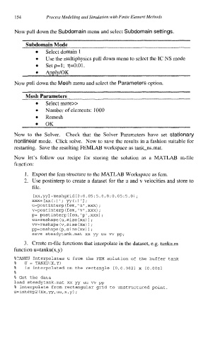
Now let's follow our recipe for storing the solution as a MATLAB m-file
function:

1. Export the fem structure to the MATLAB Workspace as fem.
2. Use postinterp to create a dataset for the u and v velocities and store to
file.
[xx,yyl =meshgrid(O: 0.05:5.0,0: 0.05 :5.0) ;
xxx=[xx(:)'; yy(:)'];
u=postinterp(fem, 'u' ,xxx) ;
v=postinterp(fem,'v',xxx);
p= postinterp(fem,'p',xxx);
uu=reshape (u, size (xx) ) ;
w=reshape (v, size (xx) ;
)
pp=reshape (p, size (xx) ;
)
save steadytank.mat xx yy uu w pp;
3. Create m-file functions that interpolate in the dataset, e.g. tanku.m
function u=tanku(x,y)
%TANKU Interpolates u from the FEM solution of the buffer tank
% U = TANKU(X,Y)
% is interpolated on the rectangle [O,O.OOZl x [0.0061
,
% Get the data
load steadytank.mat xx yy uu w pp
% Interpolate from rectangular grid to unstructured point
u=interp2 (xx,yy,uu,x,y)
;