Page 168 - Process Modelling and Simulation With Finite Element Methods

Extended Multiphysics 155

The tanku.m, tankv.m, and tankp.m m-file functions are now callable from
FEMLAB's GUI as initial conditions for the tank. The velocity profile is a
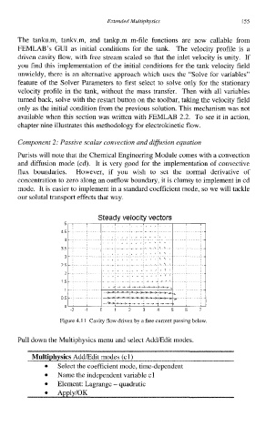
driven cavity flow, with free stream scaled so that the inlet velocity is unity. If
you find this implementation of the initial conditions for the tank velocity field
unwieldy, there is an alternative approach which uses the "Solve for variables"
feature of the Solver Parameters to first select to solve only for the stationary
velocity profile in the tank, without the mass transfer. Then with all variables
turned back, solve with the restart button on the toolbar, taking the velocity field
only as the initial condition from the previous solution. This mechanism was not
available when this section was written with FEMLAB 2.2. To see it in action,
chapter nine illustrates this methodology for electrokinetic flow.

Component 2: Passive scalar convection and diffusion equation

Purists will note that the Chemical Engineering Module comes with a convection
and diffusion mode (cd). It is very good for the implementation of convective
flux boundaries. However, if you wish to set the normal derivative of
concentration to zero along an outflow boundary, it is clumsy to implement in cd
mode. It is easier to implement in a standard coefficient mode, so we will tackle
our solutal transport effects that way.

5 ,
45 - ._ -.
4-
35-
3-
25-
2-
- . c - -_--
15- ,.
"__-_+---lJ
1- - -
e-
r
,-=ks
05- --**
A>--- + - f - * - - .>
0 '
Pull down the Multiphysics menu and select AddEdit modes.

Multiphysics Add/Edit modes (cl)
Select the coefficient mode, time-dependent
Name the independent variable cl
Element: Lagrange - quadratic
0 Apply/OK