Page 18 - Process Modelling and Simulation With Finite Element Methods

Introduction to FEMLAB 5

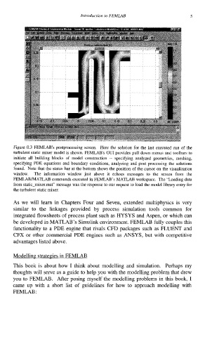
Figure 0.3 FEMLAB’s postprocessing screen. Here the solution for the last executed run of the
turbulent static mixer model is shown. FEMLAB’s GUI provides pull down menus and toolbars to
initiate all building blocks of model construction -- specifying analyzed geometries, meshing,
specifying PDE equations and boundary conditions, analyzing and post processing the solutions
found. Note that the status bar at the bottom shows the position of the cursor on the visualization
window. The information window just above it echoes messages to the screen from the
FEMLABMATLAB commands executed in FEMLAB’s MATLAB workspace. The “Loading data
from static-mixer.mat” message was the response to our request to load the model library entry for
the turbulent static mixer.

As we will learn in Chapters Four and Seven, extended multiphysics is very
similar to the linkages provided by process simulation tools common for
integrated flowsheets of process plant such as HYSYS and Aspen, or which can
be developed in MATLAB’s Simulink environment. FEMLAB fully couples this
functionality to a PDE engine that rivals CFD packages such as FLUENT and
CFX or other commercial PDE engines such as ANSYS, but with competitive
advantages listed above.

Modelling. strategies in FEMLAB
This book is about how I think about modelling and simulation. Perhaps my
thoughts will serve as a guide to help you with the modelling problem that drew
you to FEMLAB. After posing myself the modelling problems in this book, I
came up with a short list of guidelines for how to approach modelling with
FEMLAB: