Page 272 - Process Modelling and Simulation With Finite Element Methods

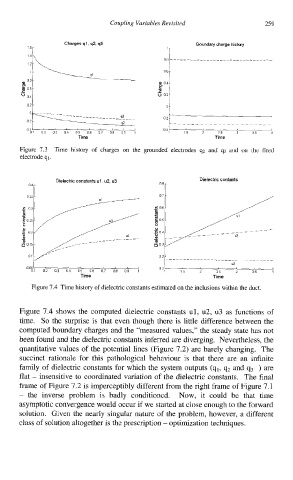
Coupling Variables Revisited 259

16- 1-
I4
06~
l : ' - . . . _ 08 ______I_
Ql
' r
@J 04-
P
io5-
u 02-
04-
02- 0-
--------_-->?__- 02-
92 ------_-__---___----_-
0 4 " " ~ " ' ~ 04
01 02 03 n4 05 06 07 08 09 I 1 15 2 25 3 35 4

Dielectric constants ul, u2, u3 Dielectric contants

0051 ' 1 ' ' L I , '
01 02 03 04 05 06 07 08 09 1
Time Time
Figure 7.4 Time history of dielectric constants estimated on the inclusions within the duct.

Figure 7.4 shows the computed dielectric constants ul, u2, u3 as functions of
time. So the surprise is that even though there is little difference between the
computed boundary charges and the "measured values," the steady state has not
been found and the dielectric constants inferred are diverging. Nevertheless, the
quantitative values of the potential lines (Figure 7.2) are barely changing. The
succinct rationale for this pathological behaviour is that there are an infinite
family of dielectric constants for which the system outputs (ql, q2 and q3 ) are
flat - insensitive to coordinated variation of the dielectric constants. The final
frame of Figure 7.2 is imperceptibly different from the right frame of Figure 7.1
- the inverse problem is badly conditioned. Now, it could be that time
asymptotic convergence would occur if we started at close enough to the forward
solution. Given the nearly singular nature of the problem, however, a different
class of solution altogether is the prescription - optimization techniques.