Page 267 - Process Modelling and Simulation With Finite Element Methods

254 Process Modelling and Simulation with Finite Element Methods

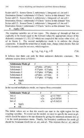
Scalar add U1. Source Geom 2, subdomain I, Integrand: ul; int ord 1
Destination Geom I subdomain 1-5 Check “Active in this domain” box.
Scalar add U2. Source Geom 2, subdomain 1, Integrand: u2; int ord 1
Destination Geom 1 subdomain 1-5 Check “Active in this domain” box.
Scalar add U3. Source Geom 2, subdomain 1, Integrand: u3; int ord 1
Destination Geom 1 subdomain 1-5 Check “Active in this domain” box.
Apply/OK

The coupling variables are of two types. The charges ql through q4 that are
explicitly to be found equal to the forward values by appropriate choice of the
dielectric constants U1, U2, U3 which are coupled to the scalar value of ul, u2,
u3 in Geom 2. The second multiphysics mode is to enforce the charge
constraints. It should be noted that at steady state, charge (total electric flux out
of the domain) must be net zero, which requires:

91 + 92 + 93 + q4 = 0 (7.6)
It follows that there can only be three unknown dielectric constants. We
arbitrary impose them as follows:

Subdomain 1 -eO*phix -eO*phiy 0 1
Subdomain 2 -U2*phix -U2*phiy 0 1
Subdomain 3 -U3*phix -U3*phiy 0 1
Subdomain 4 -e4*phix -e4*phiy 0 1
Subdomain 5 -Ul*phix -Ul*phiy 0 1
Apply

In the second multiphysics mode, we impose three constraints

Subdomain Mode gl r F da
Init e 1 -ulx ql-0,77067 1
Init e2 -u2x q2+0.30704 1
Init e3 -u3x q3+0.165 18 1
Apply
OK

The initial values are so that the search can start in the right region for the
coupling variables. To round out the model, we need to specify the mesh in 82,
which should be taken to be one element by giving the minimum element size as
1 in the mesh parameters menu. Finally, the boundary conditions for mode g2
should be Neumann (G=O) for ul, u2, and u3. This imposes that ul, u2, and u3