Page 264 - Process Modelling and Simulation With Finite Element Methods

Coupling Variables Revisited 25 1

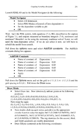
Launch FEMLAB and in the Model Navigator do the following:

Select 2-D dimension
Select PDE Modes-GenerabTime-dependent >>
Set the dependent variable as phi

Wait. Isn’t the PDE system, with equations (7.1), BCs described in the caption
of Figure 7.1, and outputs measured as boundary integrals (7.4), stationary and
nonlinear? Shouldn’t we be using the stationary nonlinear solver? Later, we will
need the time-dependent solver. If we do not select it now, we will have to
rebuild the model from scratch.

Pull down the options menu and select Add/Edit constants. The AddEdit
constants dialog box appears.

Add/Edit Constants _ _ _ _ - ~ -
Name of constant: eO Expression: 1
Name of constant: el Expression: 0.05
Name of constant: e2 Expression: 0.05
Name of constant: e3 Expression: 0.05
Name of constant: e4 Expression: 0.05
0
Apply
OK
Pull down the Options menu and set the grid to (-1.1,l.l) x (-1.1,l.l) and the
grid spacing to 0.1,O.l. Pull down the Draw menu.

Draw Mode
-___l__
Select Draw Arc. Now laboriously add arc points at the following
positions:
(0,1),(0.2,1),(0.4,0.8),(0.6,0.8),(0.8,0.6),( 1,0.4),(1,0),
( 1 ,-0.4),(0.8,-0.6),(0.6,-0. 8),(0.8,-0.6),(0.4,-0.8),(0.2,-
l),
Now swap the signs
(0,- 1),(-0.2,-1),(-0.4,-0.8), ),(-0.6,-0.8),(-0.8,-0.6),(- 1 ,-0.4),(-1 ,0),
l),
(-1,0.4),(-0.8,0.6),(-0.6,0.8),(-0.8,0.6),(-0.4,0.8),(-0.2,
Now double click on each vertex and edit it to the appropriate
circular function value for angles 5d12 (0.258819,0.965926), 4d12
(0.5,0.866025), 3d12 (0.707107,0.707107), 2d12 (0.866025, OS),
7d12 (0.965926, 0.258819). The trig identities for the second, third,
and fourth quadrants are readily determined.
Draw Ellipse (centered) at the following coordinates: