Page 266 - Process Modelling and Simulation With Finite Element Methods

Coupling Variables Revisited 253
Pull down the Solver menu and select Solver Parameters. Click on the
Settings button under “Scaling of variables.” Check the None option. Now
select the Stationary Nonlinear solver, and solve.

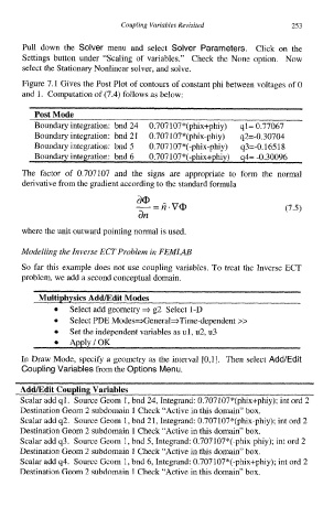
Figure 7.1 Gives the Post Plot of contours of constant phi between voltages of 0
and 1. Computation of (7.4) follows as below:

Post Mode
Boundary integration: bnd 24 0.707107*(phix+phiy) ql= 0.77067
Boundary integration: bnd 21 0.707107*(phix-phiy) q2=-0.30704
Boundary integration: bnd 5 0.707 107*(-phix-phiy) q3=-0.165 18

The factor of 0.707107 and the signs are appropriate to form the normal
derivative from the gradient according to the standard formula

(7.5)
dn
where the unit outward pointing normal is used.

Modelling the Inverse ECT Problem in FEMLAB
So far this example does not use coupling variables. To treat the Inverse ECT
problem, we add a second conceptual domain.

MultiDhvsics AddEdit Modes
Select add geometry * g2 Select 1-D
Select PDE ModesqGeneral3Time-dependent >>
Set the independent variables as ul, u2, u3
Apply/OK

In Draw Mode, specify a geometry as the interval [0,1]. Then select Add/Edit
Coupling Variables from the Options Menu.

Add/Edit Coupling Variables
Scalar add ql. Source Geom 1, bnd 24, Integrand: 0.707107*(phix+phiy); int ord 2
Destination Geom 2 subdomain 1 Check “Active in this domain” box.
Scalar add q2. Source Geom 1, bnd 21, Integrand: 0.707107*(phix-phiy); int ord 2
Destination Geom 2 subdomain 1 Check “Active in this domain” box.
Scalar add q3. Source Geom 1, bnd 5, Integrand: 0.707107*(-phix-phiy); int ord 2
Destination Geom 2 subdomain 1 Check “Active in this domain” box.
Scalar add q4. Source Geom 1, bnd 6, Integrand: 0.707107*(-phix+phiy); int ord 2
Destination Geom 2 subdomain 1 Check “Active in this domain” box.