Page 262 - Process Modelling and Simulation With Finite Element Methods

Coupling Variables Revisited 249

The image reconstruction process yields an image of the concentration
distribution within the pipe by the use of a back-projection algorithm. Existing
algorithm techniques for ECT are capable of producing images at a frame rate of
100 images per second and can, virtually, provide almost real-time information
about the process. However, a limiting feature of the existing ECT system is the
modest spatial resolution (about one tenth of the pipe radius). The major reason
for this constraint is that the surface area of each electrode is large enough that,
for all practical purposes, the electric field lines are parallel between the
electrode pairs in the chargeldischarge cycle. This convenience permits an easy
image reconstruction by the back-projection algorithm. If more and smaller
electrodes are used, there is the possibility of greater spatial resolution, but at the
cost of a more complicated reconstruction algorithm. This algorithm would need
to solve a Poisson equation with boundary data to find the internal permittivity
field.
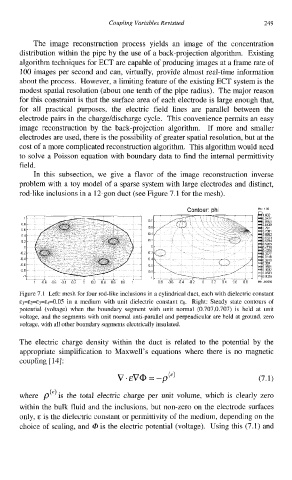
In this subsection, we give a flavor of the image reconstruction inverse
problem with a toy model of a sparse system with large electrodes and distinct,
rod-like inclusions in a 12-gon duct (see Figure 7.1 for the mesh).

Contour phi
oa
06
04
02
0
02
04
06
08 08
1 1
1 oa 06 04 02 o 02 04 06 oa I 08 06 04 02 0 02 04 06 08
Figure 7.1 Left: mesh for four rod-like inclusions in a cylindrical duct, each with dielectric constant
in
&1=&~=&3=&4=0.05 a medium with unit dielectric constant a. Right: Steady state contours of
potential (voltage) when the boundary segment with unit normal (0.707,0.707) is held at unit
voltage, and the segments with unit normal anti-parallel and perpendicular are held at ground, zero
voltage, with all other boundary segments electrically insulated.
The electric charge density within the duct is related to the potential by the
appropriate simplification to Maxwell's equations where there is no magnetic
coupling [14]:

where p(')is the total electric charge per unit volume, which is clearly zero
within the bulk fluid and the inclusions, but non-zero on the electrode surfaces
only, E is the dielectric constant or permittivity of the medium, depending on the
choice of scaling, and 0 is the electric potential (voltage). Using this (7.1) and