Page 274 - Process Modelling and Simulation With Finite Element Methods

Coupling Variables Revisited 261

.
'dl', 21,. .
'intorder',4, ...
'context', 'local');
% Integrate on subdomains
...
q3=postint(fem,'-0.707107*phix-0.707107*phiy',
'cont', 'internal', ...
'contorder',2, ...
'edim' , 1, . . .
'sohum', 1, . . .
'phase', 0,. . .
.
' geomnum ,1, . .
'
'dl', 5, ...
'intorder',4, ...
'context','local');
% Integrate on subdomains
...
q4=postint(fem,'-0.707107*phix+0.707107*phiy',
'cont', 'internal', ...
'contorder',2, ...
'edim', 1,. . .
,
'solnum' 1, . . .
'phase', 0, ...
'geomnum',l, ...
'dl', 6, ...
'intorder',4, ...
'context','local');
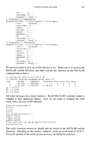
We are now ready to give our m-file function a test. Make sure it is saved in the
MATLAB current directory, and then execute the function on the MATLAB
command line as below:
>> [ql,q2,q31 =ect2 (0.05,O. 05,O. 05)
** Several warning messages print here **
Iter ErrEst Damping Stepsize nfun njac nfac nbsu
1 2e-014 1.0000000 3.1 2 1 1 2
2 1.2e-016 1.0000000 8.7e-015 3 2 2 4
ql = 0.7707
92 =-0.3070
93 =-0.1654
The error messages are a minor nuisance. Recall MATLAB's standard output is
rounded to four significant figures. Now we are ready to compute the error
norm, with a succinct m-file function:
function b=errornm(v) ;
x=v(l) ;
y=v(2) ;
z=v(3);
[ql, ~~2,931 =ect2 (x,y, z) ;
x=ql-0.77067;
y=q2+0.30704;
z=q3+0.16538;

The m-file function err0rnm.m should also be stored in the MATLAB current
directory. Checking on the known "solution" yields an error norm of O(10-5).
Given the sparsity of the mesh, greater accuracy would not be expected.