Page 279 - Process Modelling and Simulation With Finite Element Methods

266 Process Modelling and Simulation with Finite Element Methods

lower intensity due to absorption by a chemical species. For dilute chemical
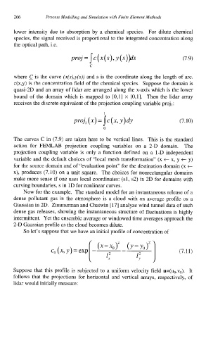
species, the signal received is proportional to the integrated concentration along
the optical path, i.e.

(7.9)

where _C is the curve (x(s),y(s)) and s is the coordinate along the length of arc.
c(x,y) is the concentration field of the chemical species. Suppose the domain is
quasi-2D and an array of lidar are arranged along the x-axis which is the lower
bound of the domain which is mapped to [0,1] x [0,1]. Then the lidar array
receives the discrete equivalent of the projection coupling variable proj ,:

(7.10)

The curves C in (7.9) are taken here to be vertical lines. This is the standard
action for FEMLAB projection coupling variables on a 2-D domain. The
projection coupling variable is only a function defined on a 1-D independent
variable and the default choices of “local mesh transformation” (x t x, y t y)
for the source domain and of “evaluation point” for the destination domain (x t
x), produces (7.10) on a unit square. The choices for nonrectangular domains
make more sense if one uses local coordinates: (sl, s2) in 2D for domains with
curving boundaries, s in 1D for nonlinear curves.
Now for the example. The standard model for an instantaneous release of a
dense pollutant gas in the atmosphere is a cloud with an average profile 0s a
Gaussian in 20. Zimmerman and Chatwin [ 171 analyze wind tunnel data of such
dense gas releases, showing the instantaneous structure of fluctuations is highly
intermittent. Yet the ensemble average or windowed time averages approach the
2-D Gaussian profile as the cloud becomes dilute.
So let’s suppose that we have an initial profile of concentration of

Suppose that this profile is subjected to a uniform velocity field u=(uo,vo). It
follows that the projections for horizontal and vertical arrays, respectively, of
lidar would initially measure: