Page 282 - Process Modelling and Simulation With Finite Element Methods

Coupling Variables Revisited 269

In Mesh mode, we need to set the symmetry boundaries as 1 4 2 3, which is
treated pairwise so that 1 and 4 are symmetry boundaries as are 2 and 3. The
combination of symmetry boundaries and boundary condition coefficients
achieves doubly periodic boundary conditions. Upon meshing, 417 elements
with 772 nodes were created in the 2-D domain.

The major action is the computation of the projection coupling variables. Select
Add/Edit Coupling Variables from the Options Menu.

AddIEdit Coupling Variables
Projection add proj 1. Source Geom 1, subdomain 1, Integrand: c; int ord 2
Local mesh transformation (x t x, y t y)
Destination Geom 1 bnd 2 Check “Active in this domain” box.
Evaluation point (x t x)
Projection add proj2. Source Geom 1, subdomain 1, Integrand: c; int ord 2
Local mesh transformation (x t y, y t x)
Destination Geom 1 bnd 1 Check “Active in this domain” box.
Evaluation point (x t x)
Amlv/OK
Set the Solver Parameters on the Solve menu with output times [0:0.001:0.06]
on the time stepping page. Select Apply/OK and hit the Solve = button on the
toolbar. After about twenty seconds of overhead computation, the time stepping
begins. As the problem is linear, it does not take long per step.
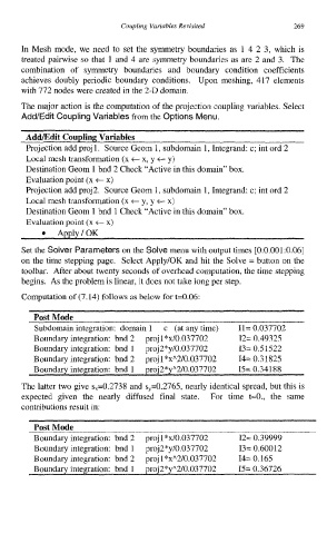
Computation of (7.14) follows as below for t=0.06:

Post Mode
Subdomain integration: domain 1 c (at any time) 11= 0.037702
Boundary integration: bnd 2 proj 1 *x/0.037702 12= 0.49325
Boundary integration: bnd 1 proj2*y/0.037702 13= 0.51522
Boundary integration: bnd 2 proj 1 *xA2/0.037702 I4= 0.31825
Boundary integration: bnd 1 proj2*yA2/0.037702 I5= 0.34188

The latter two give s,=0.2738 and s,=0.2765, nearly identical spread, but this is
expected given the nearly diffused final state. For time t=O., the same
contributions result in:

Post Mode
Boundary integration: bnd 2 pr0.j l*x/0.037702 12= 0.39999
Boundary integration: bnd 1 pr42*y/0.037702 13= 0.60012
Boundary integration: bnd 2 proj 1 *xA2/0.037702 14= 0.165
Boundary integration: bnd I proj2*yA2/0.037702 I5= 0.36726