Page 283 - Process Modelling and Simulation With Finite Element Methods

270 Process Modelling and Simulation with Finite Element Methods

MBX 0752 Max 0 0513
Time=O 001 Contour concentration of c Time.0 06 Contour concentration ofc
07163 I' I 0 0501
0 6805 0 0489
0 6447 0 0 0477 0466
0 6089
0 5731
0 5373 0 0453
0 M4l
0
043
0 5014
0 4656
0 4298 0 0418
0 0406
0 394 0 0394
0 3552 0 0382
3224
0
0
037
0 28s5 0 0358
0 2507 0 0346
02149 0 0334
031
0 1791 0 0 0322
01433
0 1075
00716
0 0238
0274
0 0358 0 0 0286
I, I
Mm 2,380, 05 0 05 1 15 hln 0 "252
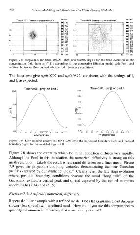
Figure 7.8 Isopycnals for times t=0.001 (left) and t=0.06 (right) for the time evolution of the
concentration field from cg (7.1 1) according to the convective-diffusion model with Pe=l and
uniform horizontal flow under doubly periodic boundary conditions.
The latter two give s,=0.0707 and s,=0.0872, consistent with the settings of 1,
and 1, as expected.
Time=0.06, projl on bnd 2 Time=0.06, proj2 on bnd 1
0 042 1
0 045 0 044 r
Q
0 035
0 034
0 032
'
'
'
0031 " " ' 1 ' " 003l " " ' ,
0 01 02 03 04 05 06 07 08 09 1 0 01 02 03 04 05 06 07 08 09 1
x-coordinate y-coordinate
Figure 7.9 Line integral projections for t=0.06 onto the horizontal boundary (left) and vertical
boundary (nght) for the model of Figure 7.8.
Figure 7.8 shows the extent to which the initial condition diffuses very rapidly.
Although the Pe=l in this simulation, the numerical diffusivity is strong on this
mesh resolution. Likely the result is less rapid diffusion on a finer mesh. Figure
7.9 gives the projection coupling variables demonstrating the near Gaussian
profiles captured by our synthetic "lidar." Clearly, even the late stage evolution
where periodic boundary conditions obscure the usual "long tails" of the
Gaussians, exhibit a central peak and spread captured by the central moments
according to (7.14) and (7.15).
Exercise 7.3: Artificial (numerical) diffusivity
Repeat the lidar example with a refined mesh. Does the Gaussian cloud disperse
slower (less spread) with a refined mesh. How could you use this computation to
quantify the numerical diffusivity that is artificially created?