Page 288 - Process Modelling and Simulation With Finite Element Methods

Coupling Variables Revisited 275

By comparison, the Subdomain settings are pedestrian:
Subdomain Mode
0 Select mode gl (geoml domain 1)
0 Set r=O, da=O, F=ul-l-eps*fl
Apply/OK
0
Select mode g2 (geom2 domain 1)
0 Set r=O 0, da=O, F=u2-f2
OK
Now for the boundary conditions. Neutral are needed. Pull down the Boundary
menu and select Boundary Settings.

Mode gl: geoml domain 1,2 Select Neumann, G=O
Mode g2: geom2 domain 1,2,3,4 Select Neumann, G=O
Apply
OK
In Mesh mode, accept the standard mesh for mode g2 (417 nodes, 772 elements)
and in mode gl, refine to 61 nodes, 60 elements. Solve. The solution should
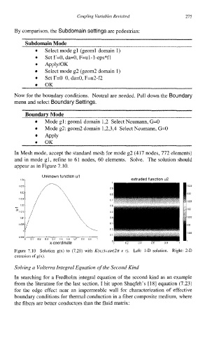
appear as in Figure 7.10.

Unknown function ul
1 04 extruded function u2

Figure 7.10 Solution g(x) to (7.20) with K(x,t)=sin(27~ x t). Left: l-D solution. Right: 2-D
extrusion of g(x).
Solving a Volterra Integral Equation of the Second Kind

In searching for a Fredholm integral equation of the second kind as an example
from the literature for the last section, I hit upon Shaqfeh’s [ 181 equation (7.23)
for the edge effect near an impermeable wall for characterization of effective
boundary conditions for thermal conduction in a fiber composite medium, where
the fibers are better conductors than the fluid matrix: