Page 293 - Process Modelling and Simulation With Finite Element Methods

280 Process Modelling and Simulation with Finite Element Methods

I
profile oftemperature gradient ul, N=l Extruded domain, contours of u2
7r I D 6095
0 6291
0 6487
0 6582
0 6878
0 7074
0 727
0 7465
0 7661
o
7857
0 8053
0 8248
0 8444
0 €64
0 8835
0 rnl
0 9227
0 9423
0 9x6
09814
1051 I ' ' ' ' ' ' ' ' ' i I ,u
0 05 1 15 2 25 3 35 4 45 5 z 2oordi;ate
z coordinate
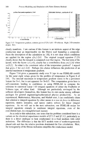
Figure 7.13 Temperature gradient, solution g(z) to (7.23). Left: 1-D solution. Right: 2-D extrusion
ofg(x). N=l.
clearly manifests. I am curious if this feature is an intrinsic aspect of the edge
conduction near an impermeable (to the fibers) wall bounding a composite.
From the description of the calculation in [18], it is not clear which conditions
are applied for the region x2~[-2,0]. The original integral equation (7.23)
clearly shows that the integral is computed over that region. The last term of the
kernel, with the factor (x+z>O), clearly has a contribution from x~[-2,0] when
z~[O,2]. So what is the consistent value of the temperature gradient? I argued
that g(x)=-I for x~(-2,0]. Perhaps this choice influences the prediction of an
internal maximum in temperature gradient.
Figure 7.14 gives a parametric study over N (eps in our FEMLAB model)
for the same eight values given for the profiles of temperature in Figure 6 of
[18]. The internal maximum in temperature gradient seems to be a persistent
feature for N>1, but is not apparent for N<0.5. The computation given here is
self-consistent, leading to confidence in using FEMLAB to compute the
solutions to canonical linear 1-D integral equations of either the Fredholm or
Volterra type, of either kind. Although not particularly envisaged by the
software developers themselves, this feature has its own niche among software
packages for general engineering/mathematical physics productivity. As an
experienced, Mathematica, Macsyma, and Matlab user, I can confidently claim
that solution to integral equations by other means is a tour de force in difference
equations, matrix assembly, and sparse matrix solvers for linear integral
equations. As we will see in the next subsection, our FEMLAB recipe for
integral equations extends to nonlinear integral equations, even of the
convolution type, in a straightforward manner.
As a coda to this subsection, one notes that the problem considered here is a
variant on the electrical capacitance models of §7.3.2 and 57.3.3, particularly as
there is a direct analogue to heat conductance in a fluid medium with solid
inclusions. The difference is that the ECT models were of nonhomogeneously
placed rods and thus the relative positions dominated the flux calculations. Here,
the homogeneity of the fibrous inclusions simplifies the conductance model.