Page 298 - Process Modelling and Simulation With Finite Element Methods

Coupling Variables Revisited 285

By comparison, the Subdomain settings are still pedestrian:

Subdomain Mode
Select mode gl (geoml domain 1)
Set r=O, da=l, F=(nl-exp(-v))/tau-ba+nl*da
0
Apply/OK
Select mode g2 (geom2 domain 1) Set r=O 0, da=O, F=n2-N1*N2
APPlY
0 OK
Now for the boundary conditions. Neutral are needed. Pull down the Boundary
menu and select Boundary Settings.

Boundarv Mode
0 Mode gl: geoml domain 1,2 Select Neumann, G=O
Mode g2: geom2 domain 1,2,3,4 Select Neumann, G=O
APPlY
0 OK
In Mesh mode, accept the standard mesh for geom2, which gives for mode g2
(415 nodes, 768 elements) and in mode gl, set number of elements per
subdomain to 1 100, to give 251 nodes, 250 elements. Solve using the
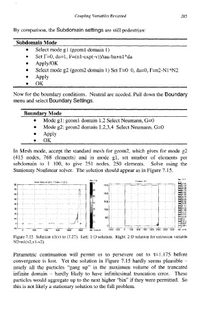
Stationaty Nonlinear solver. The solution should appear as in Figure 7.15.

COIDl oaia “I (“I) Y Data “1 (“1)
80
70
60
m
40
30
m
10
0
10
o 5m moo 1500 moo 25m
Figure 7.15 Solution nl(v) to (7.27). Left: l-D solution. Right: 2-D solution for extrusion variable
N2=nl (v2,vl-v2).
Parametric continuation will permit us to persevere out to ~=1.175 before
convergence is lost. Yet the solution in Figure 7.15 hardly seems plausible -
nearly all the particles “gang up” in the maximum volume of the truncated
infinite domain - hardly likely to have infinitesimal truncation error. These
particles would aggregate up to the next higher “bin” if they were permitted. So
this is not likely a stationary solution to the full problem.