Page 299 - Process Modelling and Simulation With Finite Element Methods

286 Process Modelling and Simulation with Finite Element Methods

“Time Dependent )’ Solution
The stationary nonlinear solution just doesn’t work. It apparently becomes ill-
posed at ~=1.175. A check of the eigenvalues suggests that the Jacobian matrix
is becoming singular - the condition number is large. It is possible that the
coupling variables are not contributing significantly to the assembly of the
stiffness matrix, which would then become singular. Iteration worked for
Nicmanis and Hounslow [27]. One way to iterate is to specify a pseudo time
scale and use the time-dependent solver. We anticipated this by putting da=l in
mode gl. For time integration, use the fldaspk solver, as it turns out the
computation is stiff. The time integration out to t=0.3 is shown in Figure 7.16.
z* 1
Time=U 3 Canfour N2
30 I 7:
2500
25 ~ 25
20 - I 20 2000
15 ~ 15
1500
10- 10
5- 1
00 I y ,.-- -,- --, __ 5
0
5- 500
10 ~ 5
11, 0 lD00 500 0 500 1000 1500 2000 25UQ 3000 3500
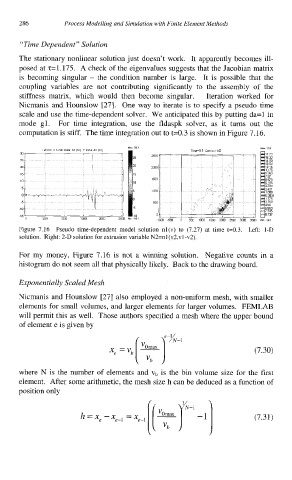
Figure 7.16 Pseudo time-dependent model solution nl(v) to (7.27) at time t=0.3. Left: 1-D
solution. Right: 2-D solution for extrusion variable N2=nl (v2,vl -v2).
For my money, Figure 7.16 is not a winning solution. Negative counts in a
histogram do not seem all that physically likely. Back to the drawing board.
Exponentially Scaled Mesh

Nicmanis and Hounslow [27] also employed a non-uniform mesh, with smaller
elements for small volumes, and larger elements for larger volumes. FEMLAB
will permit this as well. Those authors specified a mesh where the upper bound
of element e is given by

(7.30)

where N is the number of elements and vb is the bin volume size for the first
element. After some arithmetic, the mesh size h can be deduced as a function of
position only