Page 297 - Process Modelling and Simulation With Finite Element Methods

284 Process Modelling and Simulation with Finite Element Methods

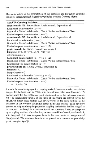
The major action is the computation of the extrusion and projection coupling
variables. Select Add/Edit Coupling Variables from the Options Menu.

AddEdit Coupling Variables
extrusion add N1. Source Geom 1, subdomain 1, Expression: nl
Local mesh transformation (x t v)
Destination Geom 2 subdomain 1, Check “Active in this domain” box.
Evaluation point transformation (x t v2)
extrusion add N2. Source Geom 1, subdomain 1, Expression: nl
Local mesh transformation (x t v)
Destination Geom 2 subdomain 1, Check “Active in this domain” box.
Evaluation point transformation (x t vl-v2)
projection add ba. Source Geom 2, subdomain 1;
*
Integrand: (v2sO) (v2<v1/2) *N1*N2
integration order 2
Local mesh transformation (x t vl , y t v2)
Destination Geom 1 subdomain 1, Check “Active in this domain” box.
Evaluation point transformation (x t v)
projection add da. Source Geom 2, subdomain 1;
Integrand: N1
integration order 2
Local mesh transformation (x t vl, y t v2)
Destination Geom 1 subdomain 1, Check “Active in this domain” box.
Evaluation point transformation (x t v)
Apply/OK
It should be noted that projection coupling variable ba computes the convolution
integral for the birth term in (7.28), with the awkward offset coordinate (vl-v2)
treated neatly by the evaluation point transformation in the extrusion variable
N2. The independent variable in the limits of integration are catered for by the
MATLAB binary logic factors (v2>O)*(v2<v1/2), in the same fashion as the
treatment of the Volterra integration limits in the last section. da is far more
pedestrian, only requiring the projection coupling variable for the line integral to
be computed. Although da is the same for all v (a constant), it must be computed
by a coupling variable. On reflection, its source could be Geom 1, subdomain 1,
with integrand nl to save computer labor in this case due to the assignment of
P(v,w)=betaO. The treatment here is more general to accommodate potentially
greater complexity of p.