Page 292 - Process Modelling and Simulation With Finite Element Methods

Coupling Variables Revisited 279
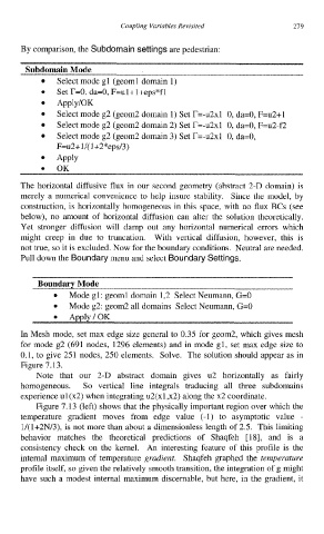
By comparison, the Subdomain settings are pedestrian:

Select mode gl (geoml domain 1)
Set r=O, da=O, F=ul+l+eps*fl
Apply/OK
Select mode g2 (geom2 domain 1) Set r=-u2xl 0, da=O, F=u2+1
Select mode g2 (geom2 domain 2) Set r=-u2xl 0, da=O, F=u2-f2
Select mode g2 (geom2 domain 3) Set r=-u2xl 0, da=O,
F=u2+ 1/( 1 +2 *eps/3)
Apply

The horizontal diffusive flux in our second geometry (abstract 2-D domain) is
merely a numerical convenience to help insure stability. Since the model, by
construction, is horizontally homogeneous in this space, with no flux BCs (see
below), no amount of horizontal diffusion can alter the solution theoretically.
Yet stronger diffusion will damp out any horizontal numerical errors which
might creep in due to truncation. With vertical diffusion, however, this is
not true, so it is excluded. Now for the boundary conditions. Neutral are needed.
Pull down the Boundary menu and select Boundary Settings.

Mode 82: geom2 all domains Select Neumann, G=O

In Mesh mode, set max edge size general to 0.35 for geom2, which gives mesh
for mode g2 (691 nodes, 1296 elements) and in mode gl, set max edge size to
0.1, to give 251 nodes, 250 elements. Solve. The solution should appear as in
Figure 7.13.
Note that our 2-D abstract domain gives u2 horizontally as fairly
homogeneous. So vertical line integrals traducing all three subdomains
experience ul (x2) when integrating u2(xl,x2) along the x2 coordinate.
Figure 7.13 (left) shows that the physically important region over which the
temperature gradient moves from edge value (-1) to asymptotic value -
1/(1+2N/3), is not more than about a dimensionless length of 2.5. This limiting
behavior matches the theoretical predictions of Shaqfeh [18], and is a
consistency check on the kernel. An interesting feature of this profile is the
internal maximum of temperature gradient. Shaqfeh graphed the temperature
profile itself, so given the relatively smooth transition, the integration of g might
have such a modest internal maximum discernable, but here, in the gradient, it