Page 289 - Process Modelling and Simulation With Finite Element Methods

276 Process Modelling and Simulation with Finite Element Methods

2
g (z)+ I+ N K (z, x)g (z + x)dx = 0 (7.23)
-2
Here, g(z) is the gradient of the ensemble average temperature at a distance z
from the edge of the wall in scaled coordinates. Shaqfeh’s theory derives the
non-local contributions for average extra flux due to the presence of randomly
positioned fibers. N is the dimensionless parameter expressing number density
and slenderness of the fibers. The kernel is given here in MATLAB notation
K(Z,X)=((X>~)*(Z~~*(~-~*X-~*Z)+(~*Z-X+~)*(X+Z-~)~~*(X+Z>~))+
(~<0)*((2*~+3 *~+2)*(~-2)~2*(~>2)+(~-2*~+6)*(~+~)~2*(~+~>0)))/12;
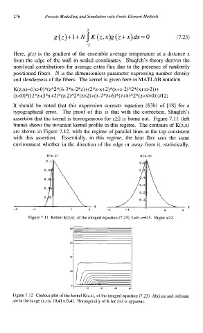
It should be noted that this expression corrects equation (83b) of [18] for a
typographical error. The proof of this is that with the correction, Shaqfeh’s
assertion that the kernel is homogeneous for 222 is borne out. Figure 7.11 (left
frame) shows the invariant kernel profile in this regime. The contours of K(z,x)
are shown in Figure 7.12, with the regime of parallel lines at the top consistent
with this assertion. Essentially, in this regime, the heat flux sees the same
environment whether in the direction of the edge or away from it, statistically,

0.1

0.0 O.A--;

I t
-2 -1 1
Figure 7.11 Kernel K(z,x), of the integral equation (7.23) Left: z=0.5. Right: 222.

Figure 7.12 Contour plot of the kernel K(z,x), of the integral equation (7.23) Abcissa and ordinate
are in the range (X,Z)E [0,4] x[O,4]. Homogeneity of K for 222 is apparent.