Page 294 - Process Modelling and Simulation With Finite Element Methods

Coupling Variables Revisited 28 1

N50
N=?O
N=lO
N5
N=3
-

N=l
NS.5
-

NS.1
I 3 a I;
LcmLdinate
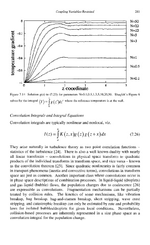
Figure 7.14 Solution g(z) to (7.23) for parameters N=0.1,0.5,1,3,5,10,20,50. Shaqfeh’s Figure 6
solves for the integral ( T ) = 5 ( zyz’ where the reference temperature is at the wall.
0

Convolution Integrals and Integral Equations
Convolution integrals are typically nonlinear and nonlocal, viz.
b
Ic,,=SK(z,x)g(z)g(z+x)~x (7.26)
a

They arise naturally in turbulence theory as two point correlation functions -
statistics of the turbulence [24]. There is also a well known duality with nearly
all linear transforms - convolutions in physical space transform to quadratic
products of the individual transforms in transform space, and vice versa - known
as the convolution theorem [25]. Since quadratic nonlinearity is fairly common
in transport phenomena (inertia and convective terms), convolutions in transform
space are just as common. Another important class where convolutions occur is
in phase space descriptions of combination processes. In liquid-liquid (droplets)
and gas-liquid (bubble) flows, the population changes due to coalescence [26]
are expressible as convolutions. Fragmentation mechanisms can be partially
treated by collision rules. The kinetics of some mechanisms, like vibration
breakup, bag breakup, bag-and-stamen breakup, sheet stripping, wave crest
stripping, and catastrophic breakup can only be estimated by rate and probability
laws for isolated bubbles/droplets for given local conditions. Nevertheless,
collision-based processes are inherently represented in a size phase space as a
convolution integral for the population change.