Page 290 - Process Modelling and Simulation With Finite Element Methods

Coupling Variables Revisited 211
and therefore, the driving force for non-local heat flux is lost. Furthermore, with
the correction, we find that K(z,x) is continuous at the origin, but has a
discontinuous slope, typical of Green’s functions in 1-D [21]. Finally, we shall
see that we reproduce results consistent with Shaqfeh’s finite difference solution
of (7.23).
It turns out that (7.23), however, is not a Fredholm integral equation at all.
Why? Because the g(z+x) dependency in the integrand is not the standard form
for a Fredholm equation. Change of variable leads to a Volterra integral
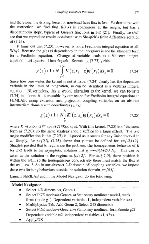
equation. Let x2=z+x. Then dxz=dx. Re-writing (7.23) yields
z+2
g(z)+l+N J K(z,x,-z)g(x,)cix, =o (7.24)

z-2
Since how one writes the kernel is not at issue, (7.24) clearly has the dependent
variable in the limits of integration, so can be identified as a Volterra integral
-
equation. Nevertheless, this a second alteration to the kernel, we can re-write
(7.24) in a form that is treatable by our recipe for Fredholm integral equations in
FEMLAB, using extrusion and projection coupling variables on an abstract
intermediate domain with coordinates (z, xz):
h
g (z ) + 1 + NJ K’ (z, x, )g (x2 ) dx, = 0 (7.25)

a
where K’=( x2>z -2)*( xz<z+2)*K(z, x2-z). With this kernel, (7.25) is of the same
form as (7.20), so the same strategy should suffice to a large extent. The one
major modification is that (7.23) is ill-posed as it stands for any finite interval in
z. Simply, for zc[O,l], (7.25) shows that g must be defined for x~[-2,1+2].
Shaqfeh posited that to regularize the problem, the homogeneous behavior of K
for z>2 leads to the asymptotic solution that g -+1/(1+2/3 N). This can be
taken as the solution in the regime x~[l,1+2]. For xe[-2,0], there position is
within the wall, so the homogeneous conductivity there must match the flux at
the wall, g=-1. So in our abstract 2-D domain of coupling variables, we impose
these two limiting behaviors outside the solution domain ZE[O,Z].
Launch FEMLAB and in the Model Navigator do the following:
Model Navigator
Select 1-D dimension, Geom 1
Select PDE modes+General=Stationary nonlinear model, weak
form (mode gl). Dependent variable ul, independent variable x>>
Multiphysics Tab. Add Geom 2, Select 2-D dimension
Select PDE modes*General+Stationary nonlinear form (mode 82)
Dependent variable u2, independent variables xl, x2>>
Apply/OK