Page 302 - Process Modelling and Simulation With Finite Element Methods

Coupling Variables Revisited 289

This will disable the solution for n2. Since it is superfluous, computing n2
can only harm us. To test how good the solution is now, we will compare
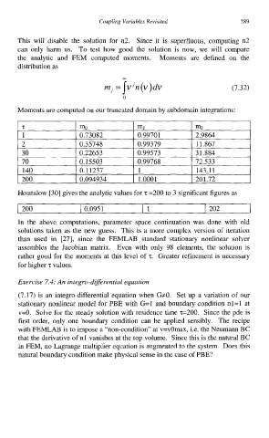
the analytic and FEM computed moments. Moments are defined on the
distribution as

(7.32)
0
Moments are computed on our truncated domain by subdomain integrations:

z 1 % I m1 I mz
1 I 0.73082 I 0.99701 1 2.9864
2 0.35748 0.99379 1 1.867
30 0.22653 0.99573 31.884
70 0.15503 0.99768 72.533
I40 0.11237 1 143.11
200 0.094934 1 .ooo 1 201.72
Hounslow [30] gives the analytic values for z =200 to 3 significant figures as

I200 I 0.0951 11 I 202
In the above computations, parameter space continuation was done with old
solutions taken as the new guess. This is a more complex version of iteration
than used in [27], since the FEMLAB standard stationary nonlinear solver
assembles the Jacobian matrix. Even with only 98 elements, the solution is
rather good for the moments at this level of 5. Greater refinement is necessary
for higher z values.

Exercise 7.4: An integro-differential equation
(7.17) is an integro-differential equation when G#O. Set up a variation of our
stationary nonlinear model for PBE with G=l and boundary condition nl=l at
v=O. Solve for the steady solution with residence time 2=200. Since the pde is
first order, only one boundary condition can be applied sensibly. The recipe
with FEMLAB is to impose a “non-condition” at v=vOmax, i.e. the Neumann BC
that the derivative of nl vanishes at the top volume. Since this is the natural BC
in FEM, no Lagrange multiplier equation is augmented to the system. Does this
natural boundary condition make physical sense in the case of PBE?