Page 375 - Process Modelling and Simulation With Finite Element Methods

362 Process Modelling and Simulation with Finite Element Methods

execute different branches of commands given that specific structure. As users
of FEMLAB, we need to know enough about the MATLAB data structure of a
FEMLAB model and solution to extract relevant data if we have particular
postprocessing or modeling requirements that are not built into the FEMLAB
GUI.

A.3 Scalar and Vector Fields: MATLAB Function Representations

Physical properties of matter typically depend on position and sometimes time.
At length scales observable to humans (by eye), most physical quantities are
treated as a continuum - having values at every mathematical point. These
quantities are called fields. Quantitites such as temperature and pressure that
represent a single value are termed scalar fields. A scalar field is a single
number, e.g.

A vector field in 3-D requires three components:

Each component of F is itself a scalar function of position.
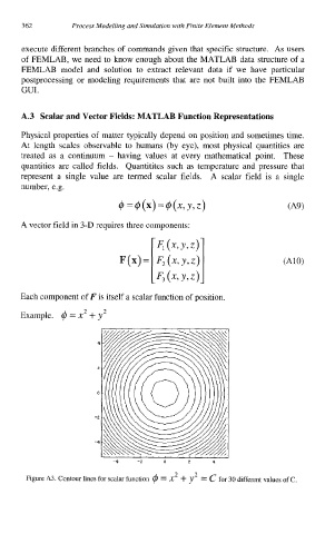
Example. @ = x2 + y2

-4 -2 0 2 4
2 2
Figure A3. Contour lines for scalar function 4 = X + Y = c for 30 different values of C.