Page 380 - Process Modelling and Simulation With Finite Element Methods

A MATLABIFEMLAB Primer for Vector Calculus 361
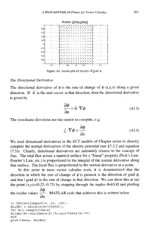
Arrow: [ ph ix, p h iy 1

-02- ' '

Figure A4. Arrow plot of vectors of grad 4

The Directional Derivative
The directional derivative of $J is the rate of change of $ (x,y,z) along a given
direction. If fi is the unit vector in that direction, then the directional derivative
is given by

The coordinate directions are the easiest to compute, e.g.

We used directional derivatives in the ECT models of Chapter seven to directly
compute the normal derivatives of the electric potential (see $7.3.2 and equation
(7.5)). Clearly, directional derivatives are intimately related to the concept of
flux. The total flux across a material surface for a "linear" property (Fick's Law,
Fourier's Law, etc.) is proportional to the integral of the normal derivative along
that surface. The local flux is proportional to the normal derivative at a point.
At this point in most vector calculus texts, it is demonstrated that the
direction in which the rate of change of q3 is greatest is the direction of grad 4,
and that I grad @ I is the rate of change in that direction. We can show this at say
the point (x,y)=(0.25,-0.75) stepping through the angles @+O,n] and plotting
by
a@
the (scalar value) - . MATLAB code that achieves this is written below.
an
>> theta=linspace(O, pi, 100) ;
)
dirder = zeros (size (theta) ;
for k=l :length (theta)
)
dirder (k) =cos (theta(k) *u+sin(theta(k) *v;
)
end
plot (theta, dirder)