Page 383 - Process Modelling and Simulation With Finite Element Methods

370 Process Modelling and Simulation with Finite Element Methods

As we saw before, the numerical approximation of derivatives is a
“primitive” of FEMLAB, so we should be able to compute approximations to
both div and curl.

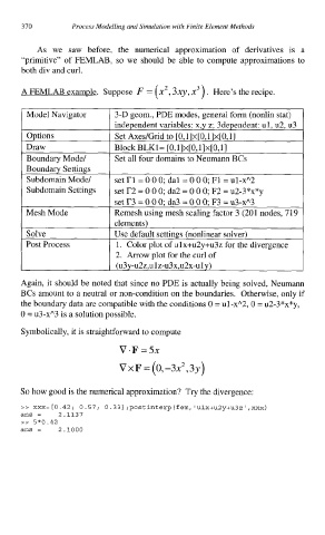
A FEMLAB example. Suppose F = (x2,3q,x3). Here’s the recipe.

Model Navigator 3-D geom., PDE modes, general form (nonlin stat)
independent variables: x,y z; 3dependent: ul, u2, u3
Options Set Axes/Grid to [O,l]x[O,llx[O,ll
Draw Block BLK1= [0,1]~[O,l]~[O,l]
Boundary Model Set all four domains to Neumann BCs
Boundary Settings
Subdomain Model set rl = 0 0 0; dal = 0 0 0; F1 = ul-xA2
Subdomain Settings set r2 = 0 0 0; da2 = 0 0 0; F2 = u~-~*x*Y
set r3 = 0 0 0; da3 = 0 0 0; F3 = u3-xA3
Mesh Mode Remesh using mesh scaling factor 3 (201 nodes, 719
elements)
Solve Use default settings (nonlinear solver)
Post Process 1. Color plot of ulx+u2y+u3z for the divergence
2. Arrow plot for the curl of
(u3y-u2z,ulz-u3x,u2x-uly)

Again, it should be noted that since no PDE is actually being solved, Neumann
BCs amount to a neutral or non-condition on the boundaries. Otherwise, only if
the boundary data are compatible with the conditions 0 = ul-xA2, 0 = u2-3*x*y,
0 = u3-xA3 is a solution possible.

Symbolically, it is straightforward to compute

VXF = (0,-3x2,3y)

So how good is the numerical approximation? Try the divergence:

>7 xxx=[O.42; 0.57; 0.33l;postinterp(fem,‘ulx+u2y+u3z’,xxx)
ans = 2.1137
>> 5*0.42
ans = 2.1000