Page 379 - Process Modelling and Simulation With Finite Element Methods

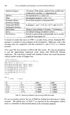
366 Process Modelling and Simulation with Finite Element Methods

Model Navigator 2-D geom., PDE modes, general form (nonlin stat)
independent variables: x,y dependent:phi
Options Set AxesIGrid to [-l,l]x[-l,l]
Draw Rectangular domain [-l,l]x[-l,l]
Boundary Model Set all four domains to Neumann BCs
Boundary Settings
Subdomain Model In domain 1, set r = 0 0; da = 0; F = phi-xA2-yA2
Subdomain Settings
Mesh Mode Remesh using default (418 nodes, 774 elements)
Solve Use default settings (nonlinear solver)
Post Process Switch to arrow mode (automatically set to vectors
I of grad @.) See Figure A4.
It should be noted that since no PDE is actually being solved, Neumann BCs
amount to a neutral or non-condition on the boundaries. Otherwise, only if the
boundary data are compatible with the condition 0 = phi-xA2-yA2 is a solution
possible.

Now export the fem structure to MATLAB (file menu). We will use postinterp
to get the approximate numerical value, along with MATLAB bilinear
regression. The code below should look familiar to those who recall the porous
catalyst (pellet) model of Chapter four.
>>x=o.5;y=o.5;
[xx,
yy] =meshgrid(-1: 0.01: 1, -1: 0.01: 1) ;
xxx= [xx : ) ' ; yy( : ) ' I ;
(
phix=postinterp(fem,'phix',xxx);
phiy=postinterp(fem,'phiy',xxx);
)
uu=reshape (phix, size (xx) ;
vv=reshape (phiy, size (xx) ;
)
u=interpZ (xx,yy,uu,x,y)
;
v=interpZ (xx,yy,w,x,y)
;
[u vl
I
ans =
1.0000 1.0000
X Y 1 phix 1 phiy
0.5 0.5 1 .oooo 1 .oooo
-0.25 0.75 -0.5000 1.5000
0.75 -0.5 1.5000 - 1 .oooo
0.25 -0.75 0.5000 -1 .so00
Table Al. Numerical estimates of grad 4 using FEMLAB model.

By any accounting method, the use of FEM for finding first derivatives is fairly
accurate. The global error of 0(10-'6) as reported in the convergence criteria
leads to a minimum of four decimal places in the estimated gradients.