Page 381 - Process Modelling and Simulation With Finite Element Methods

368 Process Modelling and Simulation with Finite Element Methods

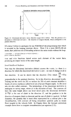
Directional derivative versus angle thee

7 7

I
'0 05 1 15 2 25 3 5
theta
Figure A5. Directional derivative versus direction (angle 0) in radians. Note the presence of a
minimum in directional derivative - the direction of steepest descent, which corresponds to the
gradient direction.

Of course I refuse to apologize for my FORTRAN-ish programming bias which
is revealed in the looping structure above. Were I in a more MATLAB-ish
mode, then judicious use of threading achieves the same results without the loop:

>>dirder = u*cos (theta) +v*sin(theta) ;
plot (theta,dirder)
cos and sin functions thread across each element of the vector theta,
producing an output vector of the same length.

Level SetdLevel Suqaces
Note that the directional derivative (dirder) crosses the x-axis, i.e. there is a
direction for which the directional derivative is zero - no rate of change at all in
a$
that direction. It can be shown that the direction hfor which -=()is
an
perpendicular to the gradient direction. So in this direction, @=constant locally.
Tracing out the curve (in 2D) or surface (in 3D) of each constant identifies a
family of curves (surfaces) called level sets of 4 (see Chapter eight). In 2D, level
sets are also called contours. The terminology of the directional derivative is
analogous to survey maps, where 4 is the elevation of land. The contours all
have the same height above sea level (level sets); the directional derivative
6 * v@ is the rate of climb in the direction 6, and the gradient is in the
direction of steepest climb (or descent) and the rate of climb is I grad 4 I. In fluid
dynamics, the quantity that is most often represented by a contour plot is the
streamfunction, with contours all being streamlines (particle paths in steady
flow) tangent to the velocity field. In Chapter three, the buoyant convection
example shows how to compute streamfunction (see equation (3.3)).