Page 377 - Process Modelling and Simulation With Finite Element Methods

3 64 Process Modelling and Simulation with Finite Element Methods
,
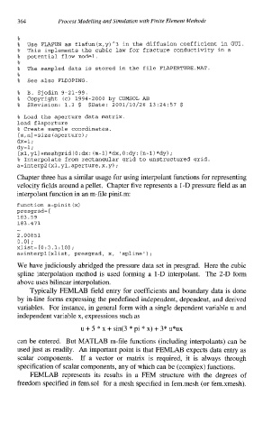
% Use FLAFUN as flafun(x,y)*3 in the diffusion coefficient in GUI.
% This implements the cubic law for fracture conductivity in a
% potential flow model.
% The sampled data is stored in the file FLAPERTURE.MAT.
%
% See also FLDOPING.
% B. Sjodin 9-21-99.
% Copyright (c) 1994-2000 by COMSOL AB
% $Revision: 1.3 $ $Date: 2001/10/26 13:24:57 $
% Load the aperture data matrix.
load flaperture
% Create sample coordinates.
[m, nl =size (aperture)
;
dx=l;
dy=l;
[xl,yl]=meshgrid(O:dx: (m-l)*dx,O:dy: (n-l)*dy)
;
% Interpolate from rectangular grid to unstructured grid.
a=interpZ(xl,yl,aperture,x,y);
Chapter three has a similar usage for using interpolant functions for representing
velocity fields around a pellet. Chapter five represents a I-D pressure field as an
interpolant function in an m-file pinit.m:
function a=pinit (XI
presgrad= [
183.59
183.471
...
2.00851
0.03;
xlist=[0:0.1:10] ;
a=interpl(xlist, presgrad, x, 'spline');
We have judiciously abridged the pressure data set in presgrad. Here the cubic
spline interpolation method is used forming a 1-D interpolant. The 2-D form
above uses bilinear interpolation.
Typically FEMLAB field entry for coefficients and boundary data is done
by in-line forms expressing the predefined independent, dependent, and derived
variables. For instance, in general form with a single dependent variable u and
independent variable x, expressions such as
u + 5 * x + sin(3 * pi * x) + 3" u*ux

can be entered. But MATLAB m-file functions (including interpolants) can be
used just as readily. An important point is that FEMLAB expects data entry as
scalar components. If a vector or matrix is required, it is always through
specification of scalar components, any of which can be (complex) functions.
FEMLAB represents its results in a FEM structure with the degrees of
freedom specified in fem.so1 for a mesh specified in fem.mesh (or fem.xmesh).