Page 71 - Process Modelling and Simulation With Finite Element Methods

58 Process Modelling and Simulation with Finite Element Methods

our example to purely Neumann conditions, you should find that the steady state
solution is 10" in size. Yet MATLAB can solve such a problem by SVD or by
the principal axis theorem. Since the matrix K is negative-semi-definite, all its
eigenvalues are real. So pseudo-inversion to eliminate the zero eigenvalue of K
follows from

>> ss=l./dd;
>> ss(l)=O.;
>> dinv=diag (ss) ;
>> uneumann=V*dinv*V'*L

Finally, interpreting this solution must be done remembering that the structure of
a FEMLAB mesh is not monotonic. These commands plot the solution:

>> [xs, idx] =sort (fem.xmesh.p {I}) ;
>>plot (xs,fem.sol.u(idx)) ;
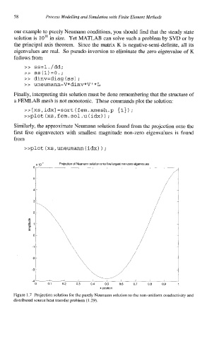
Similarly, the approximate Neumann solution found from the projection onto the
first five eigenvectors with smallest magnitude non-zero eigenvalues is found
from
>>plot(xs,uneumann(idx));

x1~3
"---- Prolection of Neumann solution onto five largest non-zero eigenvalues
v
7
1
-
-

x position
Figure 1.7 Projection solution for the purely Neumann solution to the non-uniform conductivity and
distributed source heat transfer problem (1.29).