Page 68 - Process Modelling and Simulation With Finite Element Methods

FEMLAB and the Basics of Numerical Analysis 55

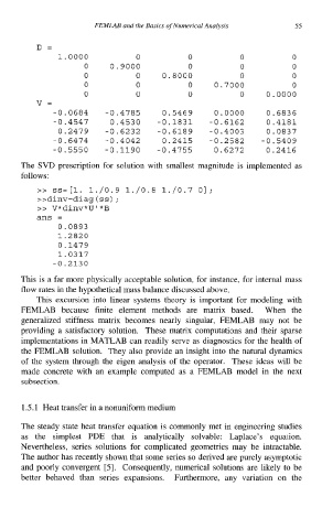
D=
1.0000 0 0 0 0
0 0.9000 0 0 0
0 0 0.8000 0 0
0 0 0 0.7000 0
0 0 0 0 0.0000
v=
-0.0684 -0.4785 0.5469 0.0000 0.6836
-0.4547 0.4530 -0.1831 -0.6162 0.4181
0.2479 -0.6232 -0.6189 -0.4003 0.0837
-0.6474 -0.4042 0.2415 -0.2582 - 0.5409
-0.5550 -0.1190 -0.4755 0.6272 0.2416
The SVD prescription for solution with smallest magnitude is implemented as
follows:
>> SS=[~. l./O.9 1./0.8 1./0.7 01;
>>dinv=diag (ss) ;
>> V*dinv*U'*B
ans =
0.0893
1.2820
0.1479
1.0317
-0.2130
This is a far more physically acceptable solution, for instance, for internal mass
flow rates in the hypothetical mass balance discussed above.
This excursion into linear systems theory is important for modeling with
FEMLAB because finite element methods are matrix based. When the
generalized stiffness matrix becomes nearly singular, FEMLAB may not be
providing a satisfactory solution. These matrix computations and their sparse
implementations in MATLAB can readily serve as diagnostics for the health of
the FEMLAB solution. They also provide an insight into the natural dynamics
of the system through the eigen analysis of the operator. These ideas will be
made concrete with an example computed as a FEMLAB model in the next
subsection.

1.5.1 Heat transfer in a nonuniform medium

The steady state heat transfer equation is commonly met in engineering studies
as the simplest PDE that is analytically solvable: Laplace's equation.
Nevertheless, series solutions for complicated geometries may be intractable.
The author has recently shown that some series so derived are purely asymptotic
and poorly convergent [5]. Consequently, numerical solutions are likely to be
better behaved than series expansions. Furthermore, any variation on the