Page 65 - Process Modelling and Simulation With Finite Element Methods

52 Process Modelling and Simulation with Finite Element Methods

time, you want to know when a determinant is zero. However, when the
determinant is zero, or numerically close to zero, it is numerically difficult to
compute due to “round-off’ swamping effects mentioned earlier. This is yet
another application for singular value decomposition.
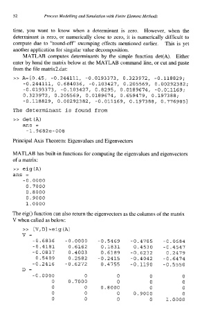
MATLAB computes determinants by the simple function det(A). Either
enter by hand the matrix below at the MATLAB command line, or cut and paste
from the file matrix2.dat:

>> A=[0.45, -0.244111, -0.0193373, 0.323972, -0.118829;
-0.244111, 0.684036, -0.103427, 0.205569, 0.00292382;
-0.0193373, -0.103427, 0.8295, 0.0189674, -0.011169;
0.323972, 0.205569, o.oia9674, 0.659479, 0.197388;
-0.118829, 0.00292382, -0.011169, 0.197388, 0.7769851
The determinant is found from
>> det(A)
ans =
-1.9682e-008
Principal Axis Theorem: Eigenvalues and Eigenvectors

MATLAB has built-in functions for computing the eigenvalues and eigenvectors
of a matrix:
>> eig(A)
ans =
-0.0000
0.7000
0.8000
0.9000
1.0000
The eig() function can also return the eigenvectors as the columns of the matrix
V when called as below:
>> [V,D] =eig (A)
v=
-0.6836 -0.0000 -0.5469 -0.4785 -0.0684
-0.4181 0.6162 0.1831 0.4530 -0.4547
-0.0837 0.4003 0.6189 -0.6232 0.2479
0.5409 0.2582 -0.2415 -0.4042 -0.6474
-0.2416 -0.6272 0.4755 -0.1190 -0.5550
D=
-0.0000 0 0 0 0
0 0.7000 0 0 0
0 0 0. aooo 0 0
0 0 0 0.9000 0
0 0 0 0 1.0000