Page 60 - Process Modelling and Simulation With Finite Element Methods

FEMLAB and the Basics of Numerical Analysis 47

Click on the triangle symbol to mesh (15 elements) and the triangle with the
embedded upside-down triangle to refine the mesh (30 elements).

Now pull down the Solve menu and select the Parameters option. This pops
up the Solver Parameters dialog window.

Solver Parameters
Select stationary linear
Solve
Cancel
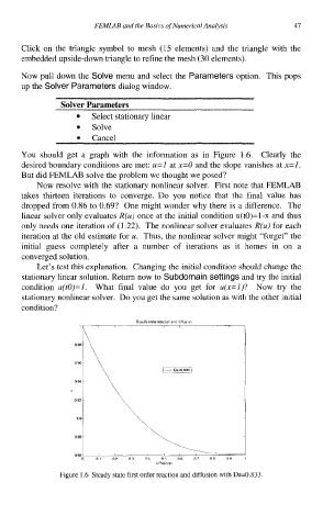
You should get a graph with the information as in Figure 1.6. Clearly the
desired boundary conditions are met: u=l at x=O and the slope vanishes at x=I.
But did FEMLAB solve the problem we thought we posed?
Now resolve with the stationary nonlinear solver. First note that FEMLAB
takes thirteen iterations to converge. Do you notice that the final value has
dropped from 0.86 to 0.69? One might wonder why there is a difference. The
linear solver only evaluates R(u) once at the initial condition u(tO)=l-x and thus
only needs one iteration of (1.22). The nonlinear solver evaluates R(u) for each
iteration at the old estimate for u. Thus, the nonlinear solver might “forget” the
initial guess completely after a number of iterations as it homes in on a
converged solution.
Let’s test this explanation. Changing the initial condition should change the
stationary linear solution. Return now to Subdomain settings and try the initial
condition u(tO)=l. What final value do you get for u(x=l)? Now try the
stationary nonlinear solver. Do you get the same solution as with the other initial
condition?

0 I \

96
1 - Da-0 833 1

id

09

01
0
088
86
0
Figure 1.6 Steady state first order reaction and diffusion with Da=0.833.