Page 63 - Process Modelling and Simulation With Finite Element Methods

50 Process Modelling and Simulation with Finite Element Methods

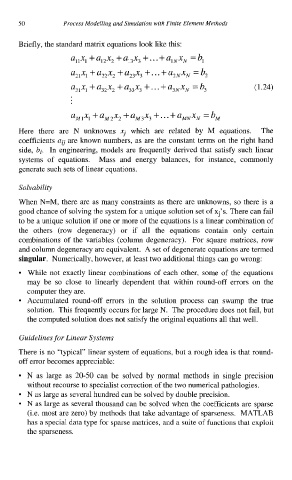
Briefly, the standard matrix equations look like this:
UllX1 + a,,x2 + q3x3 +. . . + u,,x, = b,

u,,x, + U,,X, + u2,x3 + . . . + u,,x, = b,
u3,x, + + u33x3 +. . . + u,,x, = b3 (1.24)

u,,x, +u,,x, +u,,x3 +...+ u,,x, =b,
Here there are N unknowns xj which are related by M equations. The
coefficients aq are known numbers, as are the constant terms on the right hand
side, bi. In engineering, models are frequently derived that satisfy such linear
systems of equations. Mass and energy balances, for instance, commonly
generate such sets of linear equations.

Solvability

When N=M, there are as many constraints as there are unknowns, so there is a
good chance of solving the system for a unique solution set of xj’s. There can fail
to be a unique solution if one or more of the equations is a linear combination of
the others (row degeneracy) or if all the equations contain only certain
combinations of the variables (column degeneracy). For square matrices, row
and column degeneracy are equivalent. A set of degenerate equations are termed
singular. Numerically, however, at least two additional things can go wrong:
While not exactly linear combinations of each other, some of the equations
may be so close to linearly dependent that within round-off errors on the
computer they are.
Accumulated round-off errors in the solution process can swamp the true
solution. This frequently occurs for large N. The procedure does not fail, but
the computed solution does not satisfy the original equations all that well.

Guidelines for Linear Systems
There is no “typical” linear system of equations, but a rough idea is that round-
off error becomes appreciable:
N as large as 20-50 can be solved by normal methods in single precision
without recourse to specialist correction of the two numerical pathologies.
N as large as several hundred can be solved by double precision.
N as large as several thousand can be solved when the coefficients are sparse
(i.e. most are zero) by methods that take advantage of sparseness. MATLAB
has a special data type for sparse matrices, and a suite of functions that exploit
the sparseness.