Page 67 - Process Modelling and Simulation With Finite Element Methods

54 Process Modelling and Simulation with Finite Element Methods

fractions in the splitters (order one), and that the solution mass flow rates are
about one million kgh for internal streams. Not likely. Yet this is the solution
proposed by a nearly singular matrix.
Singular Value Decomposition (SVD)

SVD offers a better solution in many respects. All matrices have a unique
decomposition, similar to the principal axis theorem for eigenvalues and
eigenvectors
A = U .diag .VT (1.26)

where U and V are square real and orthogonal. diag is a diagonal matrix which
contains the singular values. In terms of U , V, and diag, the system (1.25) is
readily solved
(1.27)

U and V being orthogonal means that their transposes are also their inverses. The
inverse of a diagonal matrix is just the reciprocal of the diagonal elements. So
the only time we have a problem solving the system is when one or more of the
singular values (diagj), relative to the largest, is close to zero. It follows that (1/
diagj) is a very large number, which distorts our numerical solution, sending it
off to infinity along a direction which is spurious. A good approximation is to
throw these spurious directions away completely by setting (1/ diagj) for the
offending singular values to zero! The vector,
(1.28)

with this substitution for nearly zero elements, should be the smallest in
magnitude to approximately satisfy the equations.

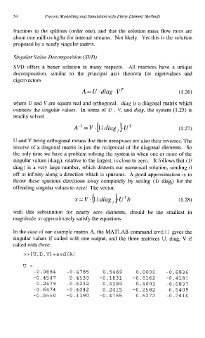
In the case of our example matrix A, the MATLAB command svd ( ) gives the
singular values if called with one output, and the three matrices U, diag, V if
called with three:
>> [U,D,V] =svd(A)
u=
-0.0684 -0.4785 0.5469 0.0000 -0.6836
-0.4547 0.4530 -0.1831 -0.6162 -0.4181
0.2479 -0.6232 -0.6189 -0.4003 -0.0837
-0.6474 -0.4042 0.2415 -0.2582 0.5409
-0.5550 -0.1190 -0.4755 0.6272 -0.2416