Page 70 - Process Modelling and Simulation With Finite Element Methods

FEMLAB and the Basics of Numerical Analysis 51

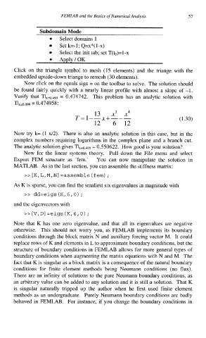
Subdomain Mode
0 Select domains 1
Set k=-1; Q=x*(l-x)
Select the init tab; set T(b)=l-x

Click on the triangle symbol to mesh (15 elements) and the triange with the
embedded upside-down triange to remesh (30 elements).
Now click on the equals sign = on the toolbar to solve. The solution should
be found fairly quickly with a nearly linear profile with almost a slope of -1.
Verify that TIx=0.499 = 0.474742. This problem has an analytic solution with
TIx4,@9 = 0.474958:

(1.30)

Now try k=-(l-x/2). There is also an analytic solution in this case, but in the
complex numbers requiring logarithms in the complex plane and a branch cut.
The analytic solution gives TIx=0.499
= 0.550622. How good is your solution?
Now for the linear systems theory. Pull down the File menu and select
Export FEM structure as ‘fem.’ You can now manipulate the solution in
MATLAB. As in the last section, you can assemble the stiffness matrix:

>> [K,L,M,N] =assemble(fem) ;
As K is sparse, you can find the smallest six eigenvalues in magnitude with
>> dd=eigs (K, 6,O) ;
and the eigenvectors with
>> [V, D] =eigs (K, 6,O) ;
Note that K has one zero eigenvalue, and that all its eigenvalues are negative
otherwise. This should not worry you, as FEMLAB implements its boundary
conditions through the block matrix N and auxiliary forcing vector M. It could
replace rows of K and elements in L to approximate boundary conditions, but the
structure of boundary conditions in FEMLAB allows for more general types of
boundary conditions when augmenting the matrix equations with N and M. The
fact that K is singular as a block matrix is a consequence of the natural boundary
conditions for finite element methods being Neumann conditions (no flux).
There are an infinity of solutions to the pure Neumann boundary conditions, as
an arbitrary value can be added to any solution and it is still a solution. That K
is singular naturally tripped up the author when he first used finite element
methods as an undergraduate. Purely Neumann boundary conditions are badly
behaved in FEMLAB. For instance, if you change the boundary conditions in