Page 64 - Process Modelling and Simulation With Finite Element Methods

FEMUB and the Basics of Numerical Analysis 51

However, in engineering and physical sciences, there are problems that by their
very nature are singular or nearly singular. You might find difficulty with N=10.
Singular value decomposition is a technique which can sometimes treat singular
problems by projecting onto non-singular ones.

Common Tasks in Numerical Linear Algebra
Equation (1.24) can be succinctly written as a matrix equation (cf. equation
1.20).
A.x=b (1.25)
Solution for the unknown vector x, where A is a square matrix of coefficients,
and b is a known vector.
Solution with more than one b vector with the matrix A held constant.
Calculation of the matrix A-I, which is the inverse of a square matrix A.
Calculation of the determinant of a square matrix A.
If M<N, or if M=N but the equations are degenerate, then there are effectively
fewer equations than unknowns-an underdetermined system. In this case,
either there can be no solution, or there is more than one solution vector x.
The solution space consists of a particular solution xp plus any linear
combination of typically N-M vectors called the nullspace of A. The task of
finding this solution space is called singular value decomposition.
If M>N, there is, in general, no solution vector x to (1.24). This
overdetermined system happens frequently, and the best compromise solution
that comes closest to satisfying the equations is sought. Usually, the closeness
is “least-squares” difference between the right and left hand sides of (1.24).

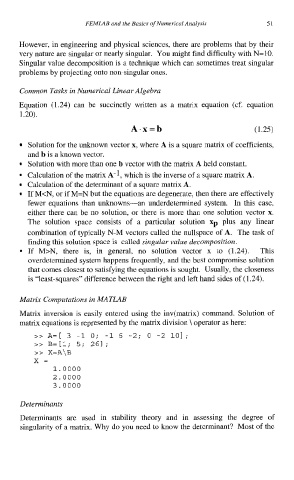
Matrix Computations in MATLAB
Matrix inversion is easily entered using the inv(matrix) command. Solution of
matrix equations is represented by the matrix division \ operator as here:
>> A=[ 3 -1 0; -1 6 -2; 0 -2 101 ;
>> B=[l; 5; 261;
>> X=A\B
x=
1.0000
2.0000
3.0000

Determinants
Determinants are used in stability theory and in assessing the degree of
singularity of a matrix. Why do you need to know the determinant? Most of the