Page 58 - Process Modelling and Simulation With Finite Element Methods

FEMLAB und the Basics of Numerical Analysis 45

values uj = u(xj) at the grid points x=xj=j Ax, then with central differences, the
system of equations becomes
L' hx2
fpl,uj =- q, Ri (1.20)
j=1 .a
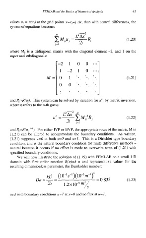
where Me is a tridiagonal matrix with the diagonal element -2, and 1 on the
super and subdiagonals:

M= (1.21)

and R,=R(uj). This system can be solved by iteration for uni by matrix inversion,
where n refers to the n-th guess:

(1.22)

and Rj=R(u '-'). For either IVP or BVP, the appropriate rows of the matrix M in
(1.21) can be altered to accommodate the boundary conditions. As written,
(1.21) supposes u=O at both x=O and x=l. This is a Dirichlet type boundary
condition, and is the natural boundary condition for finite difference methods -
natural because it occurs if no effort is made to overwrite rows of (1.21) with
specified boundary conditions.
We will now illustrate the solution of (1.19) with FEMLAB on a small 1-D
domain with first order reaction R(u)=k u and representative values for the
resulting dimensionless parameter, the Damkohler number:

-- -.-I- (1.23)
3

and with boundary conditions u=l at x=O and no flux at u=l.