Page 131 - Rapid Learning in Robotics

8.2 The Inverse 6 D Robot Kinematics Mapping 117

by little (double sized) cross-marks in the perspective view of the Puma's
workspace.

r
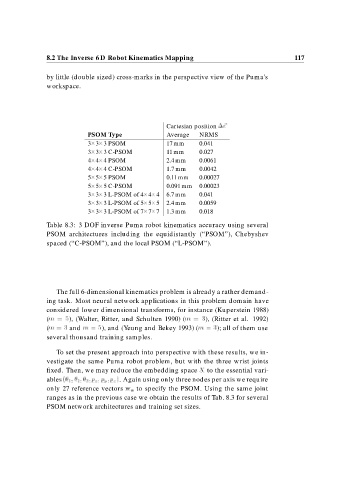
Cartesian position
PSOM Type Average NRMS
3 3 3 PSOM 17 mm 0.041
3 3 3 C-PSOM 11 mm 0.027
4 4 4 PSOM 2.4 mm 0.0061
4 4 4 C-PSOM 1.7 mm 0.0042
5 5 5 PSOM 0.11 mm 0.00027
5 5 5 C-PSOM 0.091 mm 0.00023
3 3 3 L-PSOM of 4 4 4 6.7 mm 0.041
3 3 3 L-PSOM of 5 5 5 2.4 mm 0.0059
3 3 3 L-PSOM of 7 7 7 1.3 mm 0.018

Table 8.3: 3 DOF inverse Puma robot kinematics accuracy using several
PSOM architectures including the equidistantly (“PSOM”), Chebyshev
spaced (“C-PSOM”), and the local PSOM (“L-PSOM”).

The full 6-dimensional kinematics problem is already a rather demand-
ing task. Most neural network applications in this problem domain have
considered lower dimensional transforms, for instance (Kuperstein 1988)
(m ), (Walter, Ritter, and Schulten 1990) (m ), (Ritter et al. 1992)

(m and m ), and (Yeung and Bekey 1993) (m ); all of them use
several thousand training samples.

To set the present approach into perspective with these results, we in-
vestigate the same Puma robot problem, but with the three wrist joints
fixed. Then, we may reduce the embedding space X to the essential vari-
ables p y p z . pAgain using only three nodes per axis we require
x
only 27 reference vectors w a to specify the PSOM. Using the same joint
ranges as in the previous case we obtain the results of Tab. 8.3 for several
PSOM network architectures and training set sizes.