Page 129 - Rapid Learning in Robotics

8.2 The Inverse 6 D Robot Kinematics Mapping 115

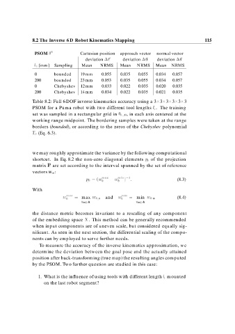
PSOM Cartesian position approach vector normal vector
r
deviation deviation a deviation n
l z [mm] Sampling Mean NRMS Mean NRMS Mean NRMS

0 bounded 19 mm 0.055 0.035 0.055 0.034 0.057
200 bounded 23 mm 0.053 0.035 0.055 0.034 0.057
0 Chebyshev 12 mm 0.033 0.022 0.035 0.020 0.035
200 Chebyshev 14 mm 0.034 0.022 0.035 0.021 0.035

Table 8.2: Full 6 DOF inverse kinematics accuracy using a 3 3 3 3 3 3
PSOM for a Puma robot with two different tool lengths l z . The training
set was sampled in a rectangular grid in , in each axis centered at the
working range midpoint. The bordering samples were taken at the range
borders (bounded), or according to the zeros of the Chebyshev polynomial
T (Eq. 6.3).

we may roughly approximate the variance by the following computational
shortcut. In Eq. 8.2 the non-zero diagonal elements p k of the projection
matrix P are set according to the interval spanned by the set of reference
vectors w a:
p k w max w min (8.3)
k
k
With

w max max w k a and w k min min w k a (8.4)
k
a A a A
the distance metric becomes invariant to a rescaling of any component

of the embedding space X. This method can be generally recommended
when input components are of uneven scale, but considered equally sig-
nificant. As seen in the next section, the differential scaling of the compo-
nents can by employed to serve further needs.

To measure the accuracy of the inverse kinematics approximation, we
determine the deviation between the goal pose and the actually attained
position after back-transforming (true map) the resulting angles computed
by the PSOM. Two further question are studied in this case:

1. What is the influence of using tools with different length l z mounted
on the last robot segment?