Page 125 - Rapid Learning in Robotics

8.1 Robot Finger Kinematics 111

4.5 10
2x2x2 used 2x2x2 used
4 equidistand spaced, full set Chebyshev spaced, full set
3x3x3 used
3x3x3 used
Mean Cartesian Deviation [mm] 2.5 3 2 Mean Cartesian Deviation [mm] 0.1 1
4x4x4 used
4x4x4 used
3.5
Chebyshev spaced, full set
equidistand spaced, full set
1.5
0.5 1
0 0.01
3 4 5 6 8 10 3 4 5 6 8 10
Knot Points per Axes Knot Points per Axes
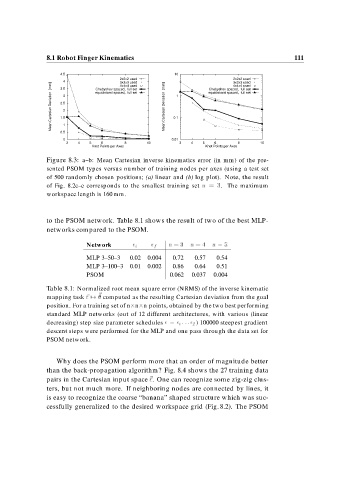
Figure 8.3: a–b: Mean Cartesian inverse kinematics error (in mm) of the pre-
sented PSOM types versus number of training nodes per axes (using a test set
of 500 randomly chosen positions; (a) linear and (b) log plot). Note, the result
of Fig. 8.2c–e corresponds to the smallest training set n . The maximum
workspace length is 160 mm.

to the PSOM network. Table 8.1 shows the result of two of the best MLP-
networks compared to the PSOM.

Network
i
f n n n

MLP 3–50–3 0.02 0.004 0.72 0.57 0.54
MLP 3–100–3 0.01 0.002 0.86 0.64 0.51
PSOM 0.062 0.037 0.004

Table 8.1: Normalized root mean square error (NRMS) of the inverse kinematic

mapping task r
computed as the resulting Cartesian deviation from the goal
position. For a training set of n n n points, obtained by the two best performing
standard MLP networks (out of 12 different architectures, with various (linear
decreasing) step size parameter schedules

i f ) 100000 steepest gradient

descent steps were performed for the MLP and one pass through the data set for
PSOM network.

Why does the PSOM perform more that an order of magnitude better
than the back-propagation algorithm? Fig. 8.4 shows the 27 training data
pairs in the Cartesian input space r. One can recognize some zig-zig clus-
ters, but not much more. If neighboring nodes are connected by lines, it
is easy to recognize the coarse “banana” shaped structure which was suc-
cessfully generalized to the desired workspace grid (Fig. 8.2). The PSOM