Page 123 - Rapid Learning in Robotics

8.1 Robot Finger Kinematics 109

the underlying transformation is highly non-linear and exhibits a point-
singularity in the vicinity of the “banana tip”. Since an analytical solution
to the inverse kinematic problem was not derived yet, this problem was
a particular challenging task for the PSOM approach (Walter and Ritter
1995).
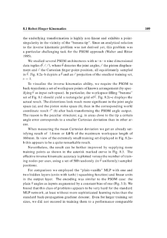
We studied several PSOM architectures with n n n nine dimensional

data tuples ( c r), where denotes the joint angles, c the piston displace-
r
ment and the Cartesian finger point position, all equidistantly sampled

r
in . Fig. 8.2a–b depicts a and an projection of the smallest training set,
n .
To visualize the inverse kinematics ability, we require the PSOM to
back-transform a set of workspace points of known arrangement (by spec-

ifying as input sub-space). In particular, the workspace filling “banana”

set of Fig. 8.1 should yield a rectangular grid of . Fig. 8.2c–e displays the
actual result. The distortions look much more significant in the joint angle
space (a), and the piston stoke space (b), than in the corresponding world

coordinate result r (b) after back-transforming the PSOM angle output.
The reason is the peculiar structure; e.g. in areas close to the tip a certain
angle error corresponds to a smaller Cartesian deviation than in other ar-
eas.
When measuring the mean Cartesian deviation we get an already sat-
isfying result of 1.6 mm or 1.0 % of the maximum workspace length of
160 mm. In view of the extremely small training set displayed in Fig. 8.2a–
b this appears to be a quite remarkable result.
Nevertheless, the result can be further improved by supplying more
training points as shown in the asterisk marked curve in Fig. 8.3. The
effective inverse kinematic accuracy is plotted versus the number of train-

ing nodes per axes, using a set of 500 randomly (in uniformly) sampled
positions.

For comparison we employed the “plain-vanilla” MLP with one and
two hidden layers (units with tanh( ) squashing function) and linear units
in the output layer. The encoding was similar to the PSOM case: the
plain angles as inputs augmented by a constant bias of one (Fig. 3.1). We
found that this class of problems appears to be very hard for the standard
MLP network, at least without more sophisticated learning rules than the
standard back-propagation gradient descent. Even for larger training set
sizes, we did not succeed in training them to a performance comparable