Page 127 - Rapid Learning in Robotics

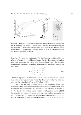
8.2 The Inverse 6 D Robot Kinematics Mapping 113

z
w
a
160
150
140 a
130
120
110
100
90

40
30 20 s
x 10 0 -10 -20 2
-30
-40 -40 -30 -20 -10 0 y 10 20 30 A∈S
r θ
s
1
Figure 8.5: The same 27 training data vectors (cmp. Fig. 8.4) for the bi-directional
PSOM mapping: (left) in the Cartesian space r, (middle) the corresponding joint

angle space . (Right:) The corresponding node locations a A in the param-
eter manifold S. Neighboring nodes are connected by lines, which reveals now
the “banana” structure on the left.

r
Here, denote the joint angles, is the Cartesian position of the end
effector of length l z in world coordinates. a and n denote the normalized
approach vector and the vector normal to the hand plane. The last nine
components vectors are part of the homogeneous coordinate transforma-
tion matrix

n x o x a x r x

n y o y a y r y
T (8.1)

n z o z a z r z

(The missing second matrix column o is the cross product of the normal-
ized orientation vectors a and n and therefore bears no further informa-
tion, see Fig. 8.6 and e.g. (Fu et al. 1987; Paul 1981).)
In this space, we must construct the m dimensional embedding
manifold M that represents the configuration manifold of the robot. With

three nodes per axis direction we require
reference vectors w a
X. The distribution of these vectors might have been found with a SOM,
however, for the present demonstration we generated the values for the
w a by augmenting 729 joint angle vectors on a rectangular 3 3 3 3 3 3

n n
grid in joint angle space with the missing r x y z r r x y a z a a x y n z –