Page 54 - Rapid Learning in Robotics

40 Artificial Neural Networks

new
old

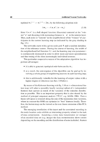
updated w a w a w a by the following adaption rule:

w a a a x h w a (3.10)

Here h a a is a bell shaped function (Gaussian) centered at the “win-

ner” a and decaying with increasing distance ja a j in the neuron layer.

Thus, each node or “neuron” in the neighborhood of the “winner” a par-
ticipates in the current learning step (as indicated by the gray shading in
Fig. 3.5.)
The networks starts with a given node grid A and a random initializa-
tion of the reference vectors. During the course of learning, the width of
the neighborhood bell function h and the learning step size parameter
is continuously decreased in order to allow more and more specialization
and fine tuning of the (then increasingly) individual neurons.
This particular cooperative nature of the adaptation algorithm has im-
portant advantages:

it is able to generate topological order between the w a;

as a result, the convergence of the algorithm can be sped up by in-
volving a whole group of neighboring neurons in each learning step;

this is additionally valuable for the learning of output values with a
higher degree of robustness (see Sect. 3.8 below).

By means of the Kohonen learning rule Eq. 3.10 an m–dimensional fea-
ture map will select a (possibly locally varying) subset of m independent
features that capture as much of the variation of the stimulus distribu-
tion as possible. This is an important property that is also shared by the
method of principal component analysis (“PCA”, e.g. Jolliffe 1986). Here a
linear sub-space is oriented along the axis of the maximum data variation,
where in contrast the SOM can optimize its “best” features locally. There-
fore, the feature map can be viewed as the non-linear extension of the PCA
method.
The emerging tessellation of the input and the associated encoding in
the node location code exhibits an interesting property related to the task
of data compression. Assuming a noisy data transmission (or storage)
of an encoded data set (e.g. image) the data reconstruction shows errors
depending on the encoding and the distribution of noise included. Feature