Page 58 - Rapid Learning in Robotics

44 The PSOM Algorithm

a a
31 33
w
Embedding 9
Space X
w Array of
3
Knots a ∈A
s 2
w
2 A∈S
s
w 1
1

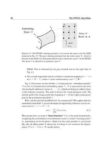
Figure 4.1: The PSOM's starting position is very much the same as for the SOM
depicted in Fig. 3.5. The gray shading indicates that the index space A , which is
discrete in the SOM, has been generalized to the continuous space S in the PSOM.
The space S is referred to as parameter space S.

PSOM. This is indicated by the grey shaded area on the right side of
Fig. 4.1.

The second important step is to define a continuous mapping w s
m
w s M X, where s varies continuously over S
IR .
Fig. 4.2 illustrates on the left the m=2 dimensional “embedded manifold”
M in the d=3 dimensional embedding space X. M is spanned by the nine
(dot marked) reference vectors w w , which are lying in a tilted plane

in this didactic example. The cube is drawn for visual guidance only. The
dashed grid is the image under the mapping w of the (right) rectangular
grid in the parameter manifold S.
How can the smooth manifold w s be constructed? We require that the
embedded manifold M passes through all supporting reference vectors w a
and write w S M X:
X
s
w s H a w a (4.1)
a A
This means that, we need a “basis function” H a s for each formal node,
weighting the contribution of its reference vector (= initial “training point”)
w a depending on the location s relative to the node position a, and possi-
bly, also all other nodes A (however, we drop in our notation the depen-
dency H a s H a s A
on the latter).