Page 60 - Rapid Learning in Robotics

46 The PSOM Algorithm

a H(a,s) a
a

s
2

s s s
1 1 1

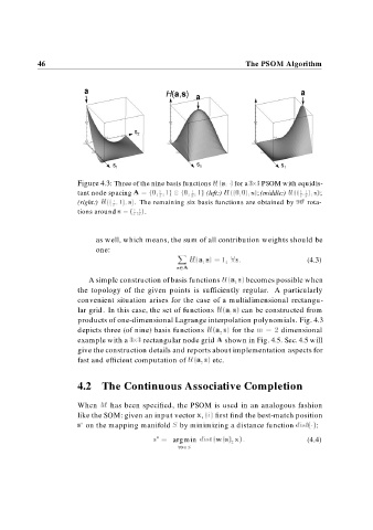
Figure 4.3: Three of the nine basis functions H a for a PSOM with equidis-
tant node spacing A f g g (left:) H s f(middle:) H s ;
;

(right:) H s . The remaining six basis functions are obtained by rota-

tions around s .

as well, which means, the sum of all contribution weights should be
one:
X
H a s s (4.3)
a A
A simple construction of basis functions H a s becomes possible when
the topology of the given points is sufficiently regular. A particularly
convenient situation arises for the case of a multidimensional rectangu-
lar grid. In this case, the set of functions H a s can be constructed from
products of one-dimensional Lagrange interpolation polynomials. Fig. 4.3
depicts three (of nine) basis functions H a s for the m dimensional
example with a rectangular node grid A shown in Fig. 4.5. Sec. 4.5 will
give the construction details and reports about implementation aspects for
fast and efficient computation of H a s etc.

4.2 The Continuous Associative Completion

When M has been specified, the PSOM is used in an analogous fashion
like the SOM: given an input vector x, i first find the best-match position

s on the mapping manifold S by minimizing a distance function dist :

s argmin dist w s x (4.4)
s S