Page 59 - Rapid Learning in Robotics

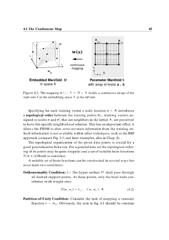
4.1 The Continuous Map 45

a a
x
3 31 33
M
w(s)
x 2

x 1 continuous
mapping s 2

w
a S
s
1
Embedded Manifold M Parameter Manifold S
in space X with array of knots a ∈ A

Figure 4.2: The mapping w S M X builds a continuous image of the
right side S in the embedding space X at the left side.

Specifying for each training vector a node location a A introduces
a topological order between the training points w a: training vectors as-

signed to nodes a and a , that are neighbors in the lattice A, are perceived
to have this specific neighborhood relation. This has an important effect: it
allows the PSOM to draw extra curvature information from the training set.
Such information is not available within other techniques, such as the RBF
approach (compare Fig. 3.3, and later examples, also in Chap. 8).
The topological organization of the given data points is crucial for a
good generalization behavior. For a general data set the topological order-
ing of its points may be quite irregular and a set of suitable basis functions
H a s difficult to construct.
A suitable set of basis functions can be constructed in several ways but
must meet two conditions:

Orthonormality Condition: i The hyper-surface M shall pass through
all desired support points. At those points, only the local node con-
tributes (with weight one):

H a i a j ij a i (4.2)
a j A

Partition-of-Unity Condition: Consider the task of mapping a constant
function x w a. Obviously, the sum in Eq. 4.1 should be constant