Page 62 - Rapid Learning in Robotics

48 The PSOM Algorithm

~ P P ~ P
A A ~ X A A A
Manifold
Manifold
Manifold
PSOM B B PSOM ~ PSOM B
X B C X
X C X C C
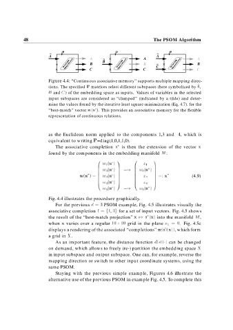
Figure 4.4: “Continuous associative memory” supports multiple mapping direc-

tions. The specified P matrices select different subspaces (here symbolized byA,

B and C) of the embedding space as inputs. Values of variables in the selected
input subspaces are considered as “clamped” (indicated by a tilde) and deter-
mine the values found by the iterative least square minimization (Eq. 4.7). for the

“best-match” vector w s . This provides an associative memory for the flexible
representation of continuous relations.

as the Euclidean norm applied to the components 1,3 and 4, which is
equivalent to writing P=diag(1,0,1,1,0).

The associative completion x is then the extension of the vector x
found by the components in the embedding manifold M:

w s x
w s w s
B C B C
B C B C
B C B C

w s B w s C B x C x (4.9)
C
B
C
B
B C B C
B w s C B x C
A A

w s w s
Fig. 4.4 illustrates the procedure graphically.
For the previous d PSOM example, Fig. 4.5 illustrates visually the
associative completion I f g for a set of input vectors. Fig. 4.5 shows

the result of the “best-match projection” x s x into the manifold M,
when x varies over a regular grid in the plane x . Fig. 4.5c

displays a rendering of the associated “completions” w s x , which form
a grid in X.
As an important feature, the distance function dist can be changed
on demand, which allows to freely (re-) partition the embedding space X
in input subspace and output subspace. One can, for example, reverse the
mapping direction or switch to other input coordinate systems, using the
same PSOM.
Staying with the previous simple example, Figures 4.6 illustrate the
alternative use of the previous PSOM in example Fig. 4.5. To complete this