Page 78 - Rapid Learning in Robotics

64 Characteristic Properties by Examples

a) X 12 X 34 b) c) X 12 X 34 d)

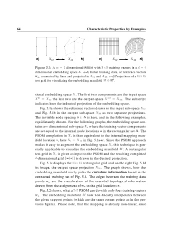
Figure 5.1: A m dimensional PSOM with
training vectors in a d
dimensional embedding space X. a–b) Initial training data, or reference vectors
w a , connected by lines and projected in X and X . c–d) Projections of a

test grid for visualizing the embedding manifold M IR .

sional embedding space X. The first two components are the input space
X in X the last two are the output-space X out X . The subscript
indicates here the indented projection of the embedding space.
Fig. 5.1a shows the reference vectors drawn in the input sub-space X
and Fig. 5.1b in the output sub-space X as two separate projections.
The invisible node spacing a A is here, and in the following examples,
equidistantly chosen. For the following graphs, the embedding space con-
tains a m dimensional sub-space X s where the training vector components

are set equal to the internal node locations a in the rectangular set A. The
PSOM completion in X s is then equivalent to the internal mapping man-
ifold location s, here X s X in Fig. 5.1a+c. Since the PSOM approach
makes it easy to augment the embedding space X, this technique is gen-
erally applicable to visualize the embedding manifold M: A rectangular
test-grid in X s is given as input to the PSOM and the resulting completed
d-dimensional grid fw s g is drawn in the desired projection.
Fig. 5.1c displays the rectangular grid and on the right Fig. 5.1d
its image, the output space projection X . The graph shows, how the
embedding manifold nicely picks the curvature information found in the
connected training set of Fig. 5.1. The edges between the training data
points w a are the visualization of the essential topological information
drawn from the assignment of w a to the grid locations a.
Fig. 5.2 shows, what a

PSOM can do with only four training vectors
w a. The embedding manifold M now non-linearly interpolates between
the given support points (which are the same corner points as in the pre-
vious figure). Please note, that the mapping is already non-linear, since