Page 85 - Rapid Learning in Robotics

5.5 Extrapolation Aspects 71

“faithfulness” of the mapping from the embedding input space to the pa-
rameter space. The topological,or “wavering” product gives an indication
on the presence of topological defects, as well as too small or too large
mapping manifold dimensionality.
As already pointed out, the PSOM draws on the curvature information
drawn from the topological order of the training data set. This information
is visualized by the connecting lines between the reference vectors w a of
neighboring nodes. How important this relative order is, is emphasized
by the shown effect if the proper order is missing, as seen Fig. 5.7.

5.5 Extrapolation Aspects

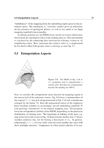
Figure 5.8: The PSOM of Fig. 5.1d in
X projection and in superposition a
second grid showing the extrapolation
beyond the training set (190 %).

Now we consider the extrapolation areas, beyond the mapping region of
the convex hull of the reference vectors. Fig. 5.8 shows a superposition of
the original test grid image presented in Fig. 5.1d and a second one
enlarged by the factor 1.9. Here the polynomial nature of the employed
basis functions exhibits an increasingly curved embedding manifold M
with growing “remoteness” to the trained mapping area. This property
limits the extrapolation abilities of the PSOM, depending on the particular
distribution of training data. The beginning in-folding of the map, e.g.
seen at the lower left corner in Fig. 5.8 demonstrates further that M shows
multiple solutions (Eq. 4.4) for finding a best-match in X . In general,
polynomials (s x) of even order (uneven node number per axes) will

show multiple solutions. Uniqueness of a best-match solution (s )isnot