Page 93 - Rapid Learning in Robotics

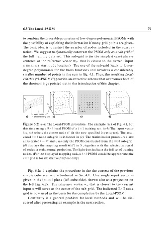
6.3 The Local-PSOM 79

to combine the favorable properties of low-degree polynomial PSOMs with
the possibility of exploiting the information if many grid points are given.
The basic idea is to restrict the number of nodes included in the compu-
tation. We suggest to dynamically construct the PSOM only on a sub-grid of
the full training data set. This sub-grid is (in the simplest case) always
centered at the reference vector w a that is closest to the current input

x (primary start node location). The use of the sub-grid leads to lower-
degree polynomials for the basis functions and involves a considerably
smaller number of points in the sum in Eq. 4.1. Thus, the resulting Local-
PSOMs (“L-PSOMs”) provide an attractive scheme that overcomes both of
the shortcomings pointed out in the introduction of this chapter.

x 3 x 3

x 3

x 2 x 2
s 2

x 2
x 2 x 1 s 1 x 1

input vector
a) best matching knot b) c) d)
Figure 6.2: a–d: The Local-PSOM procedure. The example task of Fig. 4.1, but
this time using a local PSOM of a training set. (a–b) The input vector

x x selects the closest node a (in the now specified input space). The asso-
ciated node sub-grid is indicated in (c). The minimization procedure starts

at its center s a and uses only the PSOM constructed from the sub-grid.

(d) displays the mapping result w s in X, together with the selected sub-grid
of nodes in orthonormal projection. The light dots indicate the full set of training
nodes. (For the displayed mapping task, a

PSOM would be appropriate; the
grid is for illustrative purpose only.)

Fig. 6.2a–d explains the procedure in the the context of the previous
simple cube scenario introduced in Sec. 4.1. One single input vector is
given in the x x plane (left cube side), shown also as a projection on
the left Fig. 6.2a. The reference vector w a that is closest to the current
input x will serve as the center of the sub-grid. The indicated node
grid is now used as the basis for the completion by the Local-PSOM.
Continuity is a general problem for local methods and will be dis-
cussed after presenting an example in the next section.